tgen::miniblog(4): random trees

This is a blog 4 of a series of blogs about algorithmic challenges I came across when creating tgen.

In this blog we will tackle:

1. Generate a uniformly random tree on vertices $[0, n)$ given some preset edges, in $\mathcal O(n)$ time.
2. Generate a skewed tree on vertices $[0, n)$ in $\mathcal O(n)$ time.

1. Uniform random tree with preset edges

Sometimes we want to force some edges to appear in the tree, for example because the test needs a specific path or star substructure. The preset edges may span several connected components; we need to connect those components into a single tree.

The key tool is the Prüfer sequence. Every labeled tree on $k$ vertices corresponds to a unique sequence of length $k-2$ with entries in $[0, k)$, and the degree of vertex $i$ in the tree is one plus its frequency in the sequence. A uniform random Prüfer sequence therefore gives a uniform random labeled tree.

When there are preset edges, the components play the role of super-vertices: we want to connect $c$ components into a tree, which requires exactly $c-1$ new edges. The new tree on $c$ super-vertices is generated via a random Prüfer sequence of length $c-2$. Larger components need to be more likely to be chosen, because they have more vertices that can be edge endpoints, so we sample each Prüfer entry with probability proportional to the component size using the alias method. For each new edge, a concrete vertex in each of its two components is then picked uniformly at random.

// c = number of components, comp_size[i] = size of component i
// component_ids[i] = list of vertex ids in component i
// many_by_distribution uses the alias method; returns i with probability proportional to comp_size[i]
std::vector<int> prufer = many_by_distribution(c - 2, comp_size);
for (auto [u, v] : edges_from_prufer(prufer))
    new_edges.emplace_back(pick(component_ids[u]), pick(component_ids[v]));

Algorithm 1: connecting components with a weighted Prüfer sequence.

Theorem 1: Algorithm 1 returns each labeled tree on $[0, n)$ that contains the given preset edges with the same probability.

Proof: Let the preset edges form $c$ components of sizes $s_0, \dots, s_{c-1}$, and write $n = \sum_i s_i$. Any labeled tree containing those edges contracts to a unique tree $T$ on the $c$ components. If $T$ has degrees $d_0, \dots, d_{c-1}$, component $i$ appears $d_i-1$ times in the Prüfer sequence of $T$.

Algorithm 1 samples each of the $c-2$ Prüfer entries independently with probability $s_i / n$ for component $i$. Tree $T$ has a unique Prüfer sequence $\sigma$, so

Each super-edge ${i,j}$ is then replaced by an edge between uniformly random vertices of those components. A fixed choice of original endpoints has probability

Multiplying, the probability of any specific labeled tree is

which does not depend on the tree. (If there are no preset edges, then $c = n$ and $s_i = 1$, so this is the uniform distribution over all $n^{n-2}$ labeled trees.)

Sampling and decoding the Prüfer sequence are $\mathcal O(c)$, and building the components is $\mathcal O(n)$, so the whole procedure runs in $\mathcal O(n)$ time.

2. Skewed tree

A uniformly random labeled tree has expected height $\Theta(\sqrt n)$ (see this comment). If the parent of $i$ is next(0, i-1), we get a classical random recursive tree, and the diameter is typically $\Theta(\log n)$. To force a star, we want that parent to be close to $0$; to force a path (a skewed tree, with endpoints $0$ and $n-1$), we want it close to $i-1$.

That bias is exactly wnext. For $e \geq 0$, wnext(i, e) is the maximum of $e+1$ independent samples of next(0, i-1) (so it is biased toward $i-1$). For $e \lt 0$, it is the minimum of $|e|+1$ samples (biased toward $0$).

int wnext(int i, int e) {
	int j = next(0, i - 1);
	if (e >= 0) {
		for (int t = 0; t < e; t++)
			j = std::max(j, next(0, i - 1));
	} else {
		for (int t = 0; t < std::abs(e); t++)
			j = std::min(j, next(0, i - 1));
	}
	return j;
}

std::vector<std::pair<int, int>> gen_skewed(int n, int e) {
	std::vector<std::pair<int, int>> edges;
	for (int i = 1; i < n; i++)
		edges.push_back({wnext(i, e), i});
	return edges;
}

Algorithm 2: skewed tree by wnext.

If $e$ is $0$, this is the uniform recursive tree. If $e$ is negative and large in absolute value, this is likely a star centered at $0$. If $e$ is large, this is likely a path with endpoints $0$ and $n-1$.

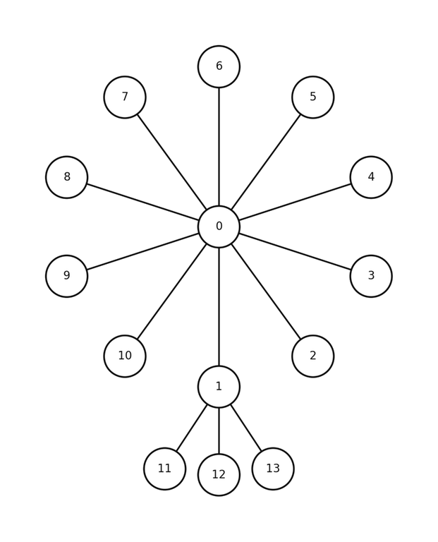
Algorithm 2 with $n = 14$ and $e = -6$ (star-like).

Algorithm 2 with $n = 14$ and $e = 6$ (path-like).

In particular, as $e$ grows, wnext(i, e) concentrates on $j = i-1$, so vertex $i$ connects to $i-1$ with probability tending to $1$. For $e \lt 0$, it concentrates on $j = 0$.

The loop above runs in $\mathcal O(|e|)$ time, which is too slow for large $|e|$. The same distribution can be sampled in $\mathcal O(1)$ by inverse transform:

int wnext(int i, int e) {
	double r = next(0.0, 1.0);
	double x;
	if (e >= 0)
		x = std::pow(r, 1.0 / (e + 1));
	else
		x = 1.0 - std::pow(r, 1.0 / (std::abs(e) + 1));
	return (int)(x * i); // in [0, i)
}

Algorithm 3: wnext in $\mathcal O(1)$ time.

Theorem 2: Algorithm 3 has the same distribution as wnext in Algorithm 2. Using it, Algorithm 2 runs in $\mathcal O(n)$ time.

Proof: Let $k = |e| + 1$, and let $r$ be uniform in $[0, 1)$. Write $U_1, \dots, U_k$ for independent uniform samples from ${0, \dots, i-1}$.

If $e \geq 0$, Algorithm 3 returns $\lfloor i r^{1/k} \rfloor$, and

which is also $\mathbb P[\max(U_1, \dots, U_k) \le j]$.

If $e \lt 0$, Algorithm 3 returns $\lfloor i(1-r^{1/k}) \rfloor$, and

which is also $\mathbb P[\min(U_1, \dots, U_k) \le j]$.

Each call is $\mathcal O(1)$, and Algorithm 2 makes $n-1$ calls.

References

Prüfer sequence (Wikipedia): https://en.wikipedia.org/wiki/Pr%C3%BCfer_sequence

Alias method (miniblog 3): https://codeforces.com/blog/entry/156111

Random recursive tree (Wikipedia): https://en.wikipedia.org/wiki/Random_recursive_tree

Height of a uniform random labeled tree: https://codeforces.com/blog/entry/95463#comment-845014

testlib wnext tree generator: https://codeforces.com/blog/entry/18291