[Tutorial] Range minimum query in O(1) with linear time construction

TL; DR

Build a sparse table over blocks of size $b = 30 \geq \log{n}$. Now we only need to answer queries of size smaller than $b$. For that, simulate a minqueue of size $b$ over the array, and store a mask of the elements that are currently active in the minqueue. Let $\text{mask[r]}$ be the minqueue mask when the simulation is at position $\text{r}$. Now we can see that, if $r-l+1 \leq b$, then query(l, r) = r - most_significant_set_bit(mask[r] & ((1<<(r-l+1))-1)).

template<typename T> struct rmq {
	vector<T> v;
	int n; static const int b = 30;
	vector<int> mask, t;

	int op(int x, int y) { return v[x] < v[y] ? x : y; }
	int msb(int x) { return __builtin_clz(1)-__builtin_clz(x); }
	int small(int r, int sz = b) { return r-msb(mask[r]&((1<<sz)-1)); }
	rmq(const vector<T>& v_) : v(v_), n(v.size()), mask(n), t(n) {
		for (int i = 0, at = 0; i < n; mask[i++] = at |= 1) {
			at = (at<<1)&((1<<b)-1);
			while (at and op(i, i-msb(at&-at)) == i) at ^= at&-at;
		}
		for (int i = 0; i < n/b; i++) t[i] = small(b*i+b-1);
		for (int j = 1; (1<<j) <= n/b; j++) for (int i = 0; i+(1<<j) <= n/b; i++)
			t[n/b*j+i] = op(t[n/b*(j-1)+i], t[n/b*(j-1)+i+(1<<(j-1))]);
	}
	T query(int l, int r) {
		if (r-l+1 <= b) return v[small(r, r-l+1)];
		int ans = op(small(l+b-1), small(r));
		int x = l/b+1, y = r/b-1;
		if (x <= y) {
			int j = msb(y-x+1);
			ans = op(ans, op(t[n/b*j+x], t[n/b*j+y-(1<<j)+1]));
		}
		return v[ans];
	}
};

Hello, Codeforces!

Here I’ll share an algorithm to solve the classic problem of Range Minimum Query (RMQ): given a static array $A$ (there won’t be any updates), we want to find, for every $\text{query(l, r)}$, the index of the minimum value of the sub-array of $A$ that starts at index $\text{l}$ and ends at index $\text{r}$. That is, we want to find $\text{query(l, r)} = \text{arg min}_{l \leq i \leq r}{\left(A[i]\right)}$. If there are more than one such indices, we can answer any of them.

I would like to thank tfg for showing me this algorithm. If you have read about it somewhere, please share the source. The only source I could find was a comment from jcg, where he explained it briefly.

Introduction

Sparse table is a well known data structure to query for the minimum over a range in constant time. However, it requires $\Theta(n \log n)$ construction time and memory. Interestingly, we can use a sparse table to help us answer RMQ with linear time construction: even though we can’t build a sparse table over all the elements of the array, we can build a sparse table over fewer elements.

To do that, let us divide the array into blocks of size $b$ and compute the minimum of each block. If we then build a sparse table over these minimums, it will cost $\mathcal{O}(\frac{n}{b} \log{\frac{n}{b}}) \subseteq \mathcal{O}(\frac{n}{b} \log{n})$. Finally, if we choose $b \in \Theta(\log n)$, we get $\mathcal{O}(n)$ time and space for construction of the sparse table!

So, if our query indices happen to align with the limits of the blocks, we can find the answer. But we might run into the following cases:

• Query range is too small, so it fits entirely inside one block:

• Query range is large and doesn’t align with block limits:

Note that, on the second case, we can use our sparse table to query the middle part (in gray). In both cases, if were able to make small queries (queries such that $r-l+1 \leq b$), we would be done.

Handling small queries

Let’s consider queries ending at the same position $r$. Take the following array $A$ and $r = 6$.

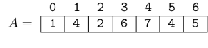
Obviously, $\text{query}(6, 6) = 6$. Since $\text{query}(5, 6) = 5 \neq \text{query}(6, 6)$, we can think of the position $\text{5}$ as “important”. Position $\text{4}$, though, is not important, because $\text{query}(4, 6) = 5 = \text{query}(5, 6)$. Basically, for fixed $r$, a position is important if the value at that position is smaller than all the values to the right of it. In this example, the important positions are $6, 5, 2, 0$. In the following image, important elements are represented with $\text{1}$ and others with $\text{0}$.

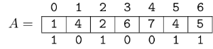
Since we only have to answer queries with size at most $b \in \Theta(\log n)$, we can store this information in a mask of size $b$: in this example $\text{mask[6] = 1010011}$, assuming $b \geq 7$. If we had these masks for the whole array, how could we figure out the minimum over a range? Well, we can simply take $\text{mask[r]}$, look at it’s $r-l+1$ least significant bits, and out of those bits take most significant one! The index of that bit would tell us how far away from $r$ the answer is.

Using our previous example, if the query was from $\text{1}$ to $\text{6}$, we would take $\text{mask[6]}$, only look at the $r-l+1=6$ least significant bits (that would give us $\text{010011}$) and out of that take the index of the most significant set bit: $\text{4}$. So the minimum is at position $r - 4 = 2$.

Now we only need to figure out how to compute theses masks. If we have some mask representing position $r$, lets change it to represent position $r+1$. Obviously, a position that was not important can’t become important, so we won’t need to turn on any bits. However, some positions that were important can stop being important. To handle that, we can just keep turning off the least significant currently set bit of our mask, until there are no more bits to turn off or the value at $r+1$ is greater than the element at the position represented by the least significant set bit of the mask (in that case we can stop, because the elements represented by important positions to the left of the least significant set bit are even smaller).

Let’s append an element with value $\text{3}$ at the end of array $A$ and update our mask.

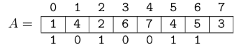
Since $\text{A[6] \gt 3}$, we turn off that bit. After that, once again $\text{A[5] \gt 3}$, so we also turn off that bit. Now we have that $\text{A[2] \lt 3}$, so we stop turning off bits. Finally, we need to append a 1 to the right of the mask, so it becomes $\text{mask[7] = 10100001}$ (assuming $b \geq 8$).

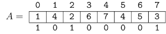
This process takes $\mathcal{O}(n)$ time: only one bit is turned on for each position of the array, so the total number of times we turn a bit off at most $n$, and using bit operations we can get and turn off the least significant currently set bit in $\mathcal{O}(1)$.

Implementation

Here is a detailed C++ implementation of the whole thing.

template<typename T> struct rmq {
	vector<T> v; int n;
	static const int b = 30; // block size
	vector<int> mask, t; // mask and sparse table

	int op(int x, int y) {
		return v[x] < v[y] ? x : y;
	}
	// least significant set bit
	int lsb(int x) {
		return x & -x;
	}
	// index of the most significant set bit
	int msb_index(int x) {
		return __builtin_clz(1)-__builtin_clz(x);
	}
	// answer query of v[r-size+1..r] using the masks, given size <= b
	int small(int r, int size = b) {
		// get only 'size' least significant bits of the mask
		// and then get the index of the msb of that
		int dist_from_r = msb_index(mask[r] & ((1<<size)-1));

		return r - dist_from_r;
	}
	rmq(const vector<T>& v_) : v(v_), n(v.size()), mask(n), t(n) {
		int curr_mask = 0;
		for (int i = 0; i < n; i++) {

			// shift mask by 1, keeping only the 'b' least significant bits
			curr_mask = (curr_mask<<1) & ((1<<b)-1);

			while (curr_mask > 0 and op(i, i - msb_index(lsb(curr_mask))) == i) {
				// current value is smaller than the value represented by the
				// last 1 in curr_mask, so we need to turn off that bit
				curr_mask ^= lsb(curr_mask);
			}
			// append extra 1 to the mask
			curr_mask |= 1;

			mask[i] = curr_mask;
		}

		// build sparse table over the n/b blocks
		// the sparse table is linearized, so what would be at
		// table[j][i] is stored in table[(n/b)*j + i]
		for (int i = 0; i < n/b; i++) t[i] = small(b*i+b-1);
		for (int j = 1; (1<<j) <= n/b; j++) for (int i = 0; i+(1<<j) <= n/b; i++)
			t[n/b*j+i] = op(t[n/b*(j-1)+i], t[n/b*(j-1)+i+(1<<(j-1))]);
	}
	// query(l, r) returns the actual minimum of v[l..r]
	// to get the index, just change the first and last lines of the function
	T query(int l, int r) {
		// query too small
		if (r-l+1 <= b) return v[small(r, r-l+1)];

		// get the minimum of the endpoints
		// (there is no problem if the ranges overlap with the sparse table query)
		int ans = op(small(l+b-1), small(r));

		// 'x' and 'y' are the blocks we need to query over
		int x = l/b+1, y = r/b-1;

		if (x <= y) {
			int j = msb_index(y-x+1);
			ans = op(ans, op(t[n/b*j+x], t[n/b*j+y-(1<<j)+1]));
		}

		return v[ans];
	}
};

But is it fast?

As you might have guessed, although the asymptotic complexity is optimal, the constant factor of this algorithm is not so small. To get a better understanding of how fast it actually is and how it compares with other data structures capable of answering RMQ, I did some benchmarks (link to the benchmark files).

I compared the following data structures. Complexities written in the notation $\lt \mathcal{O}(f), \mathcal{O}(g) \gt$ means that the data structure requires $\mathcal{O}(f)$ construction time and $\mathcal{O}(g)$ query time.

• RMQ 1 (implementation of RMQ described in this post): $\lt \mathcal{O}(n), \mathcal{O}(1) \gt$;
• RMQ 2 (different algorithm, implementation by catlak_profesor_mfb, from this blog): $\lt \mathcal{O}(n), \mathcal{O}(1) \gt$;
• Sparse Table: $\lt \mathcal{O}(n \log n), \mathcal{O}(1) \gt$;
• Sqrt-tree (tutorial and implementation from this blog by gepardo): $\lt \mathcal{O}(n \log \log n), \mathcal{O}(1) \gt$;
• Standard Segment Tree (recursive implementation): $\lt \mathcal{O}(n), \mathcal{O}(\log n) \gt$;
• Iterative (non recursive) Segment Tree: $\lt \mathcal{O}(n), \mathcal{O}(\log n) \gt$.

The data structures were executed with array size $10^6$, $2 \times 10^6$, $\dots , 10^7$. At each one of these array sizes, build time and the time to answer $10^6$ queries were measured, averaging across 10 runs. The codes were compiled with $\text{O2}$ flag. Below are the results on my machine.

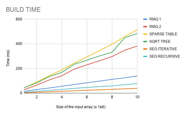
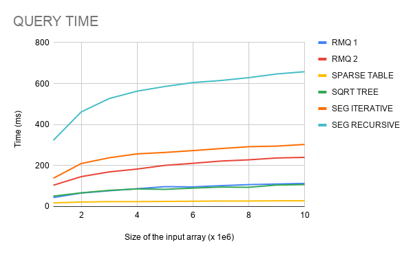
Results in table form

Build time (ms):

Query time for $10^6$ queries (ms):

Conclusion

We have an algorithm with optimal complexity to answer RMQ, and it is also simple to understand and implement. With the benchmark made, we can see that its construction is much faster than Sparse Table and Sqrt-tree, but a little slower than Segment Trees. Its query time seems to be roughly the same as Sqrt-tree, losing only to Sparse Table, which have shown to be the fastest in query time.