tgen::miniblog(7): random simple polygons

This is blog 7 of a series of blogs about algorithmic challenges I came across when creating tgen.

In this blog we will tackle:

1. Given $n$ distinct points that are not all collinear, order them as the vertices of a random simple polygon, in $\mathcal O(n\log n)$ expected time.

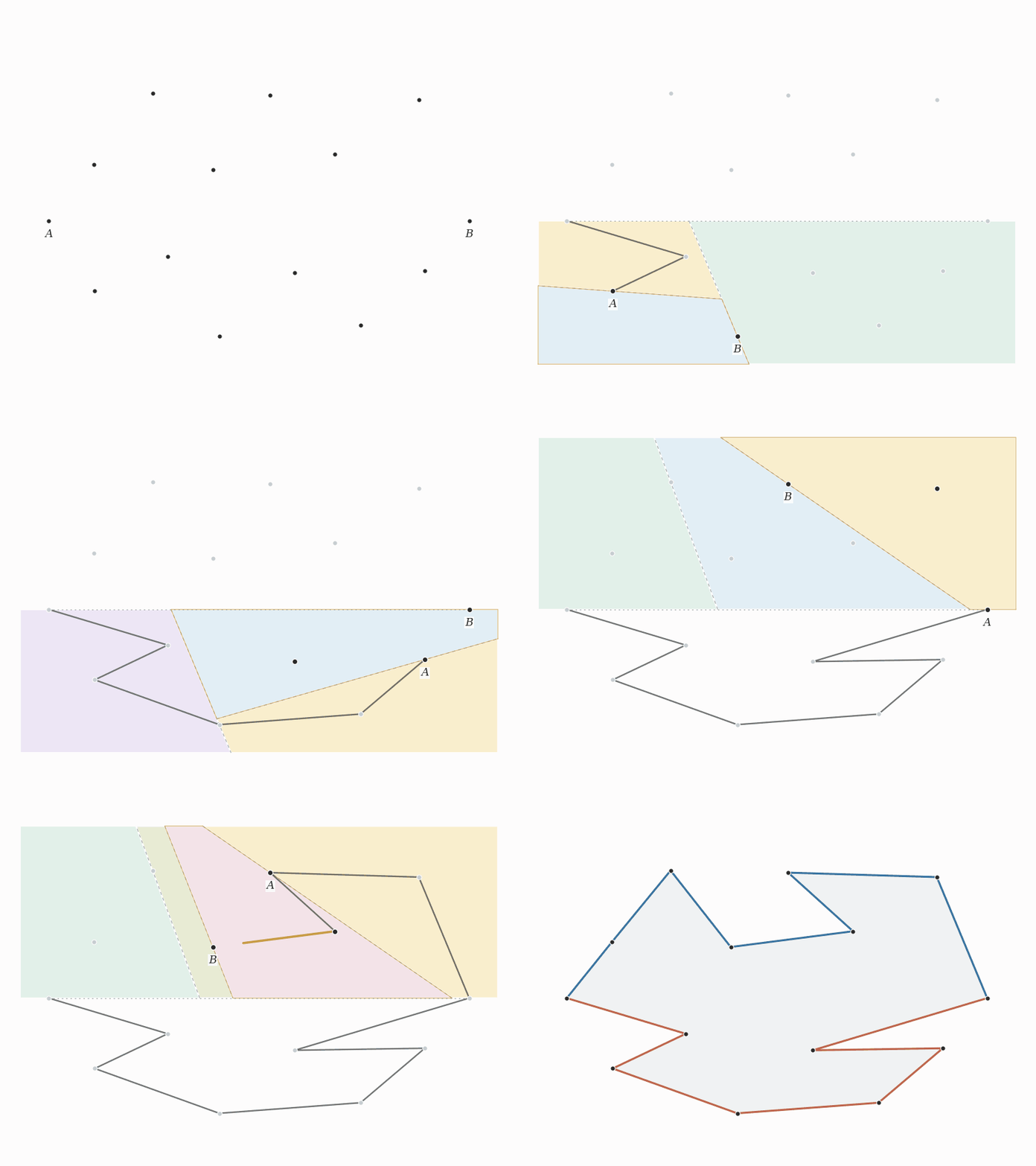
Building a simple polygon by recursively splitting the points.

A polygon is simple if its boundary does not intersect itself. A random permutation of the points usually has many crossings, and repeatedly removing crossings by local fixes can be slow. Instead, we will use divide and conquer to construct a noncrossing Hamiltonian path, then use this construction to build the polygon. I first saw this idea in this Codeforces comment.

The result is not uniformly random among all simple polygons through the points. Random choices only give us varied polygon shapes.

Using paths to create a polygon

For now, assume the points are in general position, meaning no three are collinear.

We first need a smaller problem: given a set of points containing two distinguished endpoints $A$ and $B$, construct a simple Hamiltonian path from $A$ to $B$ through every point in the set.

Suppose we can solve that problem. To build a polygon, take the lexicographically smallest point $A$ and largest point $B$. Split every other point by which side of the directed line $AB$ it lies on. Build one path from $A$ to $B$ through the points below $AB$, and another from $B$ to $A$ through the points above it.

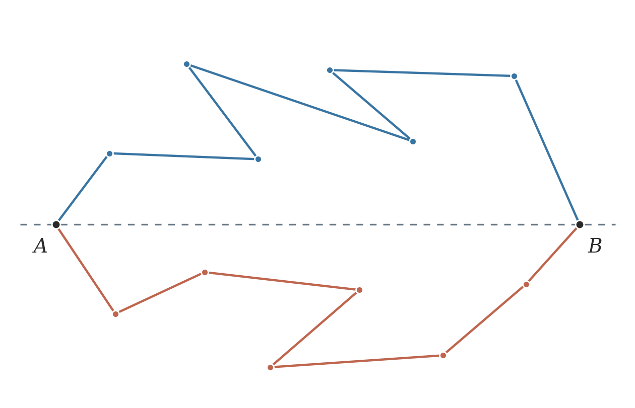
The red path runs from $A$ to $B$ below the dashed line $AB$; the blue path returns from $B$ to $A$ above it.

Since the edges of the two paths stay on opposite sides of the dividing line, the paths meet only at their endpoints $A$ and $B$. Together they form a simple polygon.

The Divide-and-Conquer Algorithm

Given a set of points and two designated endpoints $A$ and $B$, we want a noncrossing path from $A$ to $B$ that visits every point exactly once. In later recursive calls, the points may lie on both sides of $AB$. If there is at most one other point, the path is immediate. Otherwise:

1. Choose a pivot $C$ uniformly among the points different from $A$ and $B$.
2. Independently choose a point $D$ uniformly from the interior of segment $AB$.
3. The line $CD$ separates $A$ from $B$. Put every remaining point on the same side as $A$ or on the same side as $B$.

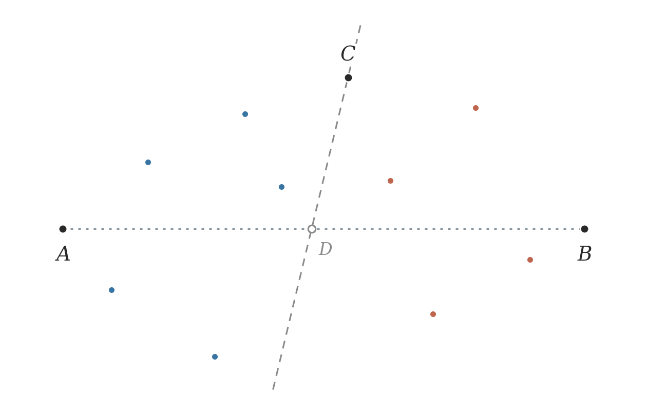
A recursive subproblem: blue points lie on the $A$-side of the dashed line $CD$, red points on the $B$-side. The hollow point $D$ lies on the dotted segment $AB$ and is not an input point.

Recursively build the path from $A$ to $C$ through the first set, and the path from $C$ to $B$ through the second set. Concatenate them at $C$ to obtain the required $A$-$B$ path.

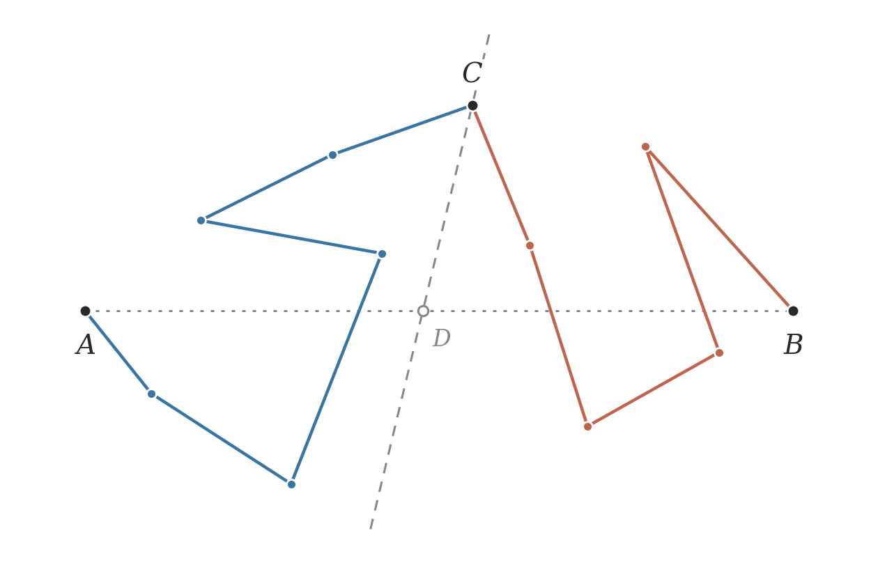
The same points after recursion. The blue $A$-$C$ path and red $C$-$B$ path stay on opposite sides of $CD$ and meet only at $C$.

There are only finitely many positions of $D$ for which $CD$ passes through another input point, so a continuous random choice avoids all of them with probability $1$.

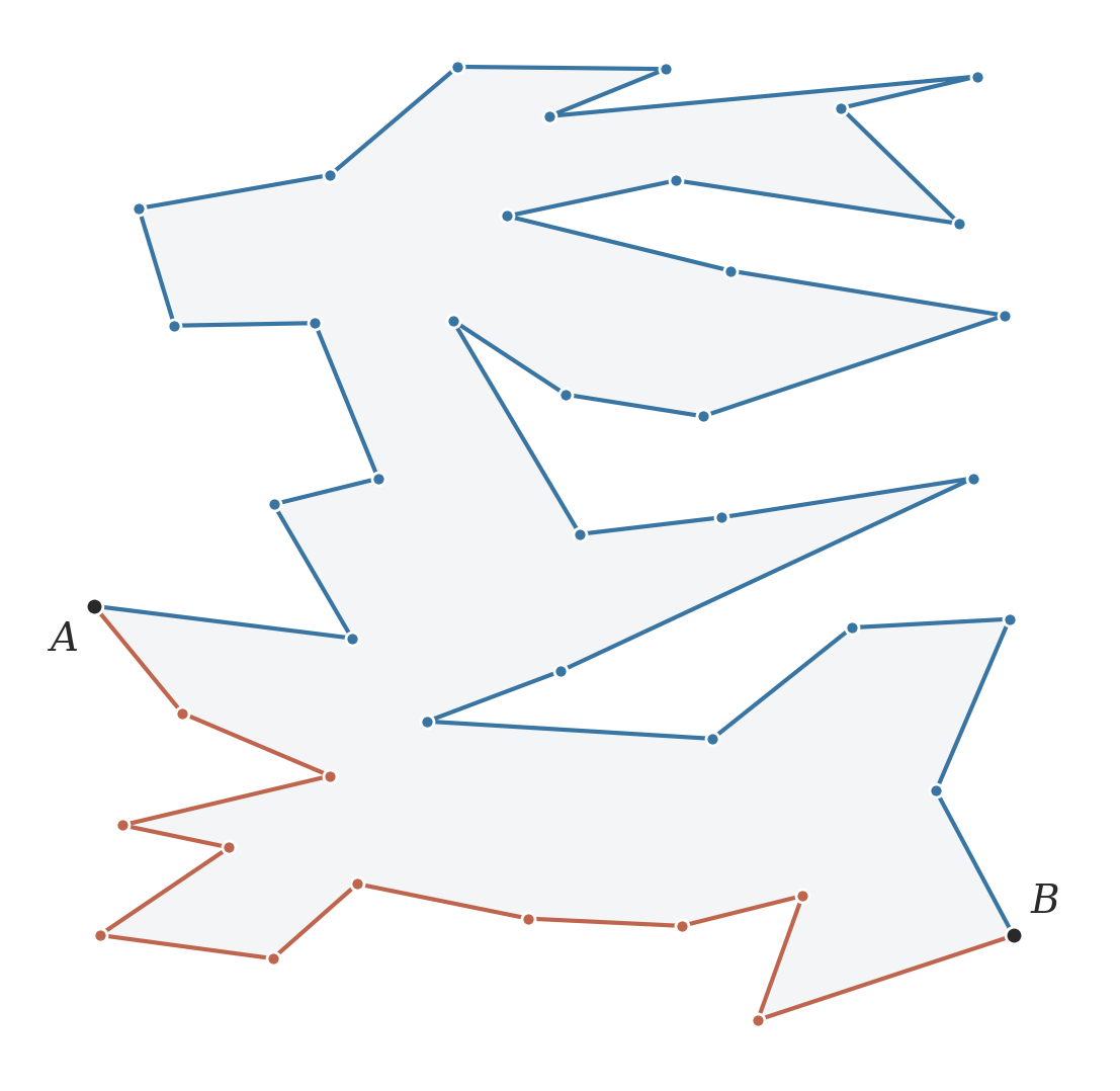
A generated polygon through 42 points. The red $A$-$B$ path and blue $B$-$A$ path form its boundary; every input point is a vertex.

Collinear points

We can also polygonize any set of at least three distinct points, as long as they are not all collinear. Consecutive edges may be collinear, but crossings and overlapping edges are still forbidden.

The construction extends to collinear inputs with some additional care; we omit those details here.

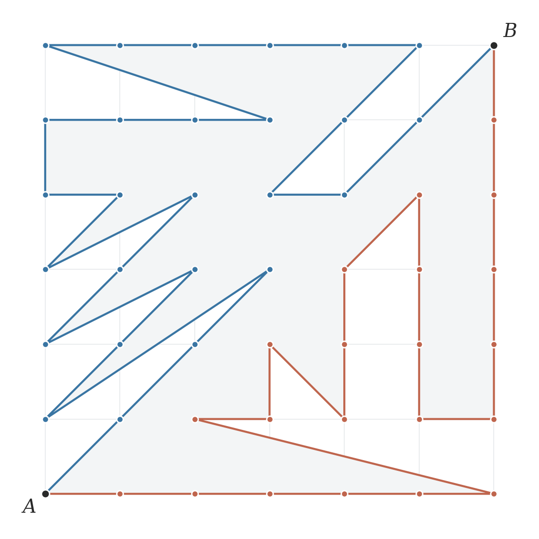
A polygonization of all 49 points of a $7\times7$ lattice. Collinear vertices are allowed; each point appears exactly once on the boundary.

Complexity

We analyze the version above with points in general position and continuous choices of $D$. The input points can be placed arbitrarily; the expectation is over the algorithm’s random choices.

Lemma 1: In a call with $m$ non-endpoint points, with probability at least $1/6$, each child has at most $5m/6$ non-endpoint points.

Proof: Fix $D$, excluding the finitely many positions that make it collinear with two non-endpoint points. Let $H$ be the points on the side of $AB$ containing the most points (choose either side in a tie). Then $k=|H|\ge m/2$. Order these points by angle around $D$.

Because $D$ lies on $AB$, these directions lie in an open semicircle. If $C$ is the $j$-th point in this order, $CD$ leaves $j-1$ points of $H$ on one side and $k-j$ on the other.

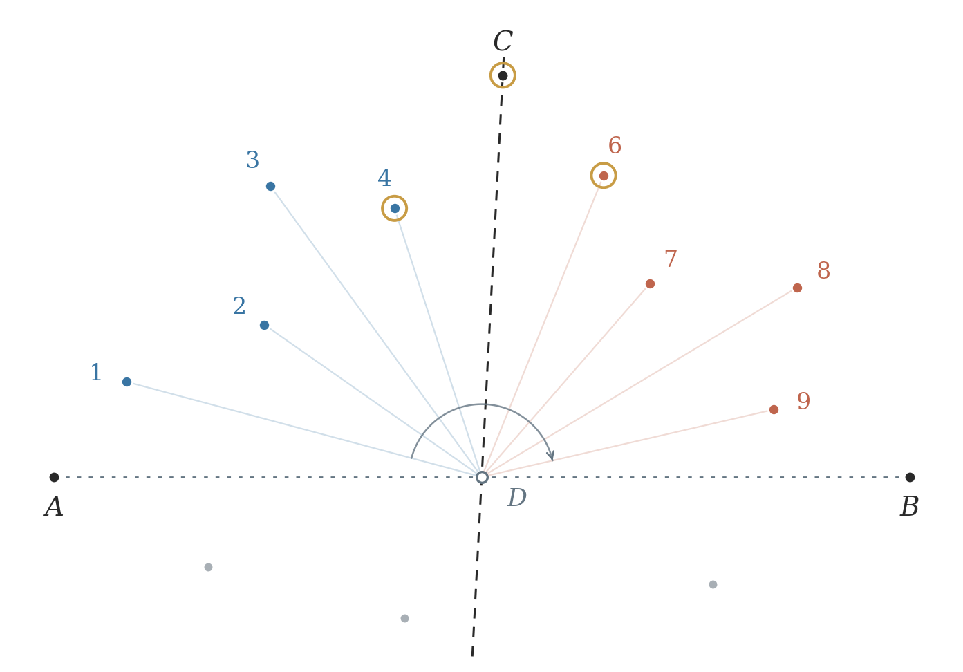
The nine points above $AB$ form $H$, numbered in angular order around $D$; the gray points are outside $H$. Here $C$ has rank $5$, so $CD$ separates four blue points from four red points. Gold rings mark ranks $4,5,6$: choosing any of these pivots leaves at least three points of $H$ on each side.

Consider pivots whose ranks in $H$ are

There are at least $k/3\ge m/6$ such pivots, so a uniform choice among all $m$ candidates selects one with probability at least $1/6$. Each side of $CD$ then contains at least $\lfloor k/3\rfloor$ points. Since $C$ becomes an endpoint of both children, either child has at most

non-endpoint points. This holds for every admissible fixed $D$, hence also for an independent continuous random choice of $D$.

$\square$

Theorem 1: For every input in general position, this version runs in $\mathcal O(n\log n)$ expected time.

Proof: Let $X_P$ count the non-base calls in which point $P$ is a non-endpoint. Call a split balanced if both children have at most $5/6$ of the parent’s non-endpoint points. Since $P$ goes to only one side of the recursion, after at most $\lceil\log_{6/5}n\rceil$ balanced splits it reaches a base case. By Lemma 1, even conditioned on previous choices, the expected wait for each balanced split (or for $P$‘s participation to end) is at most $6$ calls. Hence

Charge each non-base call’s linear work equally to its non-endpoint points. The initial split and all base calls cost $\mathcal O(n)$, so the total running time $T$ satisfies

$\square$

The expected $\mathcal O(n\log n)$ bound also extends to collinear inputs. We omit the additional case analysis to keep the proof short. An unlucky sequence of unbalanced splits can still take $\Theta(n^2)$ time.

The output distribution is not uniform, and the divide-and-conquer structure may bias which polygon shapes appear. As with any specialized generator, it is best combined with other test families when the polygon shape can affect the difficulty of the problem.

References

Thomas Auer and Martin Held, Heuristics for the Generation of Random Polygons, CCCG 1996, pp. 38–43. See “Space Partitioning” in Section 2.2, page 40.

Codeforces explanation by TLE